Julia is about two things: functions and data — and they are separate.

Everything in Julia is either a fairly straightforward function, or data.

Types

We encountered a few types in the last section, let's take a look in more detail

julia> using About

julia> about(1.0)
Float64 (<: AbstractFloat <: Real <: Number <: Any), occupies 8B.

 0011111111110000000000000000000000000000000000000000000000000000 
 ╨└────┬────┘└────────────────────────┬─────────────────────────┘
 +    2^0   ×                1.000000000000000000                
 = 1.0000000000000000

julia> about(1)
Int64 (<: Signed <: Integer <: Real <: Number <: Any), occupies 8B.

 0000000000000000000000000000000000000000000000000000000000000001
 = +1

julia> about(true)
Bool (<: Integer <: Real <: Number <: Any), occupies 1B.

 00000001 = true

julia> about((1,2, "asdf", "😠"))
Tuple{Int64, Int64, String, String} (<: Any)
 Memory footprint: 32B directly (referencing 56B in total)
 1::Int64  8B 00000000000000000000 … 00000000000000000001 1
 2::Int64  8B 00000000000000000000 … 00000000000000000010 2
 3::String 8B @ 0x00007f32f1985018                        "asdf"
 4::String 8B @ 0x00007f32f1985098                        "😠"

 ■■■■■■■■■■■■■■■■■■■■■■■■■■■■■■■■■■■■■■■■■■■■■■■■■■■■■■■■■■■■■■■■
        8B              8B              *               *        

 * = Pointer (8B)

julia> about([1,2,3,4])
4-element Vector{Int64} (mutable) (<: DenseVector{Int64} <: AbstractVector{Int64} <: Any), occupies 24B directly (referencing 72B in total, holding 32B of data)
  ref::MemoryRef{Int64} 16B «struct» MemoryRef{Int64}(Ptr … 1960), [1, 2, 3, 4])
 size::Tuple{Int64}      8B «struct» (4,)

 ■■■■■■■■■■■■■■■■■■■■■■■■■■■■■■■■■■■■■■■■■■■■■■■■
               16B                      8B       
 Int64 contents exist on the CPU within the ref::MemoryRef from 0x00007f32f8171960 to 0x00007f32f8171980.

 ┌─────────────────────── ⋯(× 4)⋯ ───────────────────────────────┐  4 items
 000000010000000000000000         00000000000000000000000000000000    in
 └─0x01─┘└─0x00─┘└─0x00─┘ ⋯(×25)⋯ └─0x00─┘└─0x00─┘└─0x00─┘└─0x00─┘ 32 bytes

julia> about([1, 1.0, "Howdy"])
3-element Vector{Any} (mutable) (<: DenseVector{Any} <: AbstractVector{Any} <: Any), occupies 24B directly (referencing 93B in total)
  ref::MemoryRef{Any} 16B «struct» MemoryRef{Any}(Ptr{No … Any[1, 1.0, "Howdy"])
 size::Tuple{Int64}    8B «struct» (3,)

 ■■■■■■■■■■■■■■■■■■■■■■■■■■■■■■■■■■■■■■■■■■■■■■■■
               16B                      8B       
 Any contents exist on the CPU within the ref::MemoryRef from 0x00007f32f3c72b40 to 0x00007f32f3c72b58.

 ┌─────────────────────── ⋯(× 3)⋯ ───────────────────────────────┐  3 pointers
 011000001001001101100011         00110010011111110000000000000000    in
 └─0x60─┘└─0x93─┘└─0x63─┘ ⋯(×17)⋯ └─0x32─┘└─0x7f─┘└─0x00─┘└─0x00─┘ 24 bytes

julia> about(rand(100))
100-element Vector{Float64} (mutable) (<: DenseVector{Float64} <: AbstractVector{Float64} <: Any), occupies 24B directly (referencing 840B in total, holding 800B of data)
  ref::MemoryRef{Float64} 16B «struct» MemoryRef{Float64}( … 0.68003, 0.281887])
 size::Tuple{Int64}        8B «struct» (100,)

 ■■■■■■■■■■■■■■■■■■■■■■■■■■■■■■■■■■■■■■■■■■■■■■■■
               16B                      8B       
 Float64 contents exist on the CPU within the ref::MemoryRef from 0x00007f32e3019c20 to 0x00007f32e3019f40.

 ┌─────────────────────── ⋯(×100)⋯ ───────────────────────────────┐ 100 items
 011010011101100100110001          01101111000010101101001000111111     in
 └─0x69─┘└─0xd9─┘└─0x31─┘ ⋯(×793)⋯ └─0x6f─┘└─0x0a─┘└─0xd2─┘└─0x3f─┘ 800 bytes

Exploring the type tree

Julia's type system is organized as a tree, with Any at the root and concrete types at the leaves. We can use AbstractTrees.jl together with subtypes to walk this hierarchy and pretty-print it:

using AbstractTrees, InteractiveUtils
AbstractTrees.children(t::Type) = subtypes(t)

Now print_tree works on any type and renders the subtype hierarchy as a textual diagram. Try it in your REPL:

julia> print_tree(Number)
Number
├─ MultiplicativeInverse
│  ├─ SignedMultiplicativeInverse
│  └─ UnsignedMultiplicativeInverse
├─ Complex
└─ Real
   ├─ AbstractFloat
   │  ├─ BigFloat
   │  ├─ BFloat16
   │  ├─ Float16
   │  ├─ Float32
   │  └─ Float64
   ├─ AbstractIrrational
   │  └─ Irrational
   ├─ Integer
   │  ├─ Bool
   │  ├─ Signed
   │  │  ├─ BigInt
   │  │  ├─ Int128
   │  │  ├─ Int16
   │  │  ├─ Int32
   │  │  ├─ Int64
   │  │  └─ Int8
   │  └─ Unsigned
   │     ├─ UInt128
   │     ├─ UInt16
   │     ├─ UInt32
   │     ├─ UInt64
   │     └─ UInt8
   └─ Rational

Tools for exploring types

The tree above gives you the shape. To poke around inside it, Julia has a small kit of reflection tools — every one works on the same Number, Real, Integer, Float64, … types you just saw.

The relations on the tree are <: (subtype) and >: (supertype):

julia> Int64 <: Integer
true

julia> Integer <: Number
true

julia> Float64 <: Integer
false

julia> Number >: Float64
true

Quiz time — dispatch-subtype: a quick subtype sanity check.

isa is the value-level version (x isa T ≡ typeof(x) <: T):

julia> 1 isa Integer
true

julia> 1.0 isa Integer
false

julia> 1.0 isa Real
true

julia> (1, 2.0) isa Tuple
true

Quiz time — dispatch-isa: the value-level companion to <:.

Walking up and down the tree:

julia> supertype(Int64)
Signed

julia> supertype(Signed)
Integer

julia> supertypes(Int64)               # full chain to Any
(Int64, Signed, Integer, Real, Number, Any)

julia> subtypes(Integer)
Any[Bool, Signed, Unsigned]

julia> subtypes(AbstractFloat)
Any[BigFloat, Core.BFloat16, Float16, Float32, Float64]

Quiz time — dispatch-supertype: walking one step up the tree.

Abstract vs. concrete — only concrete types can have instances:

julia> isabstracttype(Number)
true

julia> isabstracttype(Int64)
false

julia> isconcretetype(Int64)
true

julia> isconcretetype(Integer)
false

Two more handy ones for reasoning about overlap:

Union{...} lets you talk about "any of these" as a single type:

julia> 1 isa Union{Int, Float64}
true

julia> "hi" isa Union{Int, Float64}
false

julia> Union{Int, Float64} <: Real     # both branches are Real
true

Field introspection — handy once your own structs get involved (the Complex type from the Number tree is a good live example):

julia> fieldnames(Complex{Float64})
(:re, :im)

julia> fieldtypes(Complex{Float64})
(Float64, Float64)

julia> fieldtype(Complex{Float64}, :re)
Float64

And to ask "what methods do I have that touch this type?":

julia> methodswith(Unsigned)
Method[rem(x::Union{Int128, Int16, Int32, Int64, Int8}, y::Unsigned) @ Base int.jl:232, rem(x::Unsigned, y::Union{Int128, Int16, Int32, Int64, Int8}) @ Base int.jl:233, rem(x::Unsigned, ::Type{Signed}) @ Base int.jl:626, <<(x::Integer, c::Unsigned) @ Base operators.jl:712, >>>(x::Integer, c::Unsigned) @ Base operators.jl:793, ^(x::BigFloat, y::Unsigned) @ Base.MPFR mpfr.jl:816, abs(x::Unsigned) @ Base int.jl:187, cld(x::Signed, y::Unsigned) @ Base div.jl:350, cld(x::Unsigned, y::Signed) @ Base div.jl:351, div(x::Signed, y::Unsigned, ::RoundingMode{:Up}) @ Base div.jl:304, div(x::Signed, y::Unsigned, ::RoundingMode{:Down}) @ Base div.jl:295, div(x::Unsigned, y::Signed, ::RoundingMode{:Up}) @ Base div.jl:308, div(x::Unsigned, y::Signed, ::RoundingMode{:Down}) @ Base div.jl:299, div(x::T, y::T, ::RoundingMode{:Down}) where T<:Unsigned @ Base div.jl:368, div(x::T, y::T, ::RoundingMode{:Up}) where T<:Unsigned @ Base div.jl:375, div(x::Unsigned, y::Union{Int128, Int16, Int32, Int64, Int8}) @ Base int.jl:230, div(x::Union{Int128, Int16, Int32, Int64, Int8}, y::Unsigned) @ Base int.jl:229, divrem(x::Unsigned, y::Union{Int128, Int16, Int32, Int64, Int8}) @ Base int.jl:240, divrem(x::Union{Int128, Int16, Int32, Int64, Int8}, y::Unsigned) @ Base int.jl:235, fld(x::Signed, y::Unsigned) @ Base div.jl:348, fld(x::Unsigned, y::Signed) @ Base div.jl:349, gcd(a::Signed, b::Unsigned) @ Base intfuncs.jl:150, gcd(a::Unsigned, b::Signed) @ Base intfuncs.jl:149, gcdx(a::Signed, b::Unsigned) @ Base intfuncs.jl:257, gcdx(a::Unsigned, b::Signed) @ Base intfuncs.jl:263, isvalid(::Type{<:AbstractChar}, c::Unsigned) @ Base.Unicode strings/unicode.jl:59, lcm(a::Signed, b::Unsigned) @ Base intfuncs.jl:152, lcm(a::Unsigned, b::Signed) @ Base intfuncs.jl:151, mod(x::T, y::T) where T<:Unsigned @ Base int.jl:297, mod(x::Union{Int128, Int16, Int32, Int64, Int8}, y::Unsigned) @ Base int.jl:289, mod(x::Unsigned, y::Signed) @ Base int.jl:293, print(io::IO, n::Unsigned) @ Base show.jl:1287, show(io::IO, n::Unsigned) @ Base show.jl:1286, sign(x::Unsigned) @ Base number.jl:163, signbit(x::Unsigned) @ Base int.jl:140, widemul(x::Unsigned, y::Signed) @ Base int.jl:841, widemul(x::Signed, y::Unsigned) @ Base int.jl:840]

Advanced: Base.isbitstype(T) tells you whether T is plain old data (stack-allocatable, no pointers) — this is the property that lets values like Int64 and Float64 sit inline inside arrays without any indirection.

julia> isbits(1), isbits(1.0), isbits("hi")
(true, true, false)

Defining your own types

Immutable structs

struct (without mutable) is the default — once constructed, fields can't be rebound:

julia> struct Point
    x::Float64
    y::Float64
end

julia> p = Point(1.0, 2.0)
Main.__FRANKLIN_1181134.Point(1.0, 2.0)

julia> p.x
1.0

julia> typeof(p)
Main.__FRANKLIN_1181134.Point

Trying to mutate a field is an error:

julia> try
    p.x = 5.0
catch e
    e
end
ErrorException("setfield!: immutable struct of type Point cannot be changed")

Warning: "Immutable" means the fields can't be rebound. If a field happens to hold a mutable value (like a Vector), the contents of that value are still mutable — only the binding is frozen.

Quiz time — dispatch-mutable: what happens when you try to rebind a struct field?

Mutable structs

Prepend mutable if you need to reassign fields after construction:

julia> mutable struct Counter
    n::Int
end

julia> c = Counter(0)
Main.__FRANKLIN_1181134.Counter(0)

julia> c.n += 1
1

julia> c.n += 1
2

julia> c
Main.__FRANKLIN_1181134.Counter(2)

Mutables are heap-allocated and compared by identity (===) by default, where immutables are compared by value:

julia> Point(1.0, 2.0) == Point(1.0, 2.0)
true

julia> Counter(0) == Counter(0)
false

Quiz time — dispatch-equality: why do the two lines above disagree?

Parametric structs

A type parameter lets one struct cover many element types — and lets the compiler specialise:

julia> struct Pair2{T}
    x::T
    y::T
end

julia> Pair2(1, 2)             # Pair2{Int}
Main.__FRANKLIN_1181134.Pair2{Int64}(1, 2)

julia> Pair2(1.0, 2.0)         # Pair2{Float64}
Main.__FRANKLIN_1181134.Pair2{Float64}(1.0, 2.0)

julia> typeof(Pair2(1, 2))
Main.__FRANKLIN_1181134.Pair2{Int64}

You can constrain the parameter with <::

julia> struct NumPair{T<:Number}
    x::T
    y::T
end

julia> NumPair(1, 2)
Main.__FRANKLIN_1181134.NumPair{Int64}(1, 2)

julia> try
    NumPair("a", "b")
catch e
    e
end
MethodError(Main.__FRANKLIN_1181134.NumPair, ("a", "b"), 0x0000000000009918)

Quiz time — dispatch-box: define your own one-field parametric struct.

Abstract types and subtyping

abstract type declares a node in the type tree — no fields, no constructor, just a label other types can sit under:

julia> abstract type Animal end

julia> struct Dog <: Animal
    name::String
end

julia> struct Cat <: Animal
    name::String
end

julia> Dog("Rex") isa Animal, Cat("Mia") isa Animal
(true, true)

Methods written against the abstract type apply to every concrete subtype:

julia> speak(a::Animal) = "$(a.name) makes a sound"
Main.__FRANKLIN_1181134.var"#speak"()

julia> speak(d::Dog)    = "$(d.name) says woof"
Main.__FRANKLIN_1181134.var"#speak"()

julia> speak(Dog("Rex"))
Rex says woof

julia> speak(Cat("Mia"))
Mia makes a sound

Quiz time — dispatch-abstract: wire up your own Vehicle <: Car hierarchy.

Singleton types (no fields)

A struct with no fields is its own type — useful as a dispatch tag (this is exactly what the rock-paper-scissors example below uses):

julia> struct Marker end

julia> Marker() === Marker()
true

Quiz time — dispatch-singleton: what does Marker() === Marker() return, and why?

Constructors

By default, every struct gets one outer constructor matching its field list. You can add more outer constructors to provide defaults or conversions:

julia> struct Celsius
    value::Float64
end

julia> # Outer constructor: build a Celsius from a Fahrenheit number

julia> Celsius(°f::Int) = Celsius((°f - 32) * 5 / 9)
Main.__FRANKLIN_1181134.Celsius

julia> Celsius(0)                # 0 °F as °C
Main.__FRANKLIN_1181134.Celsius(-17.77777777777778)

julia> Celsius(100.0)            # already °C
Main.__FRANKLIN_1181134.Celsius(100.0)

An inner constructor lives inside the struct block. It's the only way to enforce invariants — you call new(...) instead of recursing into the type, and the default constructor is suppressed once you write one:

julia> struct PositiveInt
    n::Int
    function PositiveInt(n::Int)
        n > 0 || throw(ArgumentError("expected positive, got $n"))
        new(n)
    end
end

julia> PositiveInt(5)
Main.__FRANKLIN_1181134.PositiveInt(5)

julia> try
    PositiveInt(-1)
catch e
    e
end
ArgumentError("expected positive, got -1")

Advanced: Parametric inner constructors use new{T}(...), and you'll often write both a "constrained" inner ctor (enforcing the invariant) and a thin outer ctor (inferring the parameter from the arguments).

Quiz time — dispatch-inner-ctor: write an inner constructor that refuses non-positive integers. (Complex.)

Visualising dispatch

A textual tree shows the type hierarchy, but it doesn't show which method Julia would actually call for a given combination of argument types. For that we can use DispatchDisplay.jl, which renders a generic function as a grid coloured by the method dispatch would select for each cell.

Following Mosè Giordano's classic post, let's encode rock-paper-scissors as multiple dispatch. play dispatches on the types Type{Rock}, Type{Paper}, … — each explicit win-rule is its own method:

julia> abstract type Shape end

julia> struct Rock     <: Shape end

julia> struct Paper    <: Shape end

julia> struct Scissors <: Shape end

julia> play(::Type{Paper}, ::Type{Rock})     = "Paper wins"
Main.__FRANKLIN_1181134.var"#play"()

julia> play(::Type{Paper}, ::Type{Scissors}) = "Scissors wins"
Main.__FRANKLIN_1181134.var"#play"()

julia> play(::Type{Rock},  ::Type{Scissors}) = "Rock wins"
Main.__FRANKLIN_1181134.var"#play"()

julia> play(::Type{T}, ::Type{T}) where {T<:Shape} = "Tie, try again"
Main.__FRANKLIN_1181134.var"#play"()

julia> play(a::Type{<:Shape}, b::Type{<:Shape}) = play(b, a)   # commutativity fallback
Main.__FRANKLIN_1181134.var"#play"()

A couple of spot-checks at the REPL:

julia> play(Type{Paper}, Type{Rock})
ERROR: MethodError: no method matching play(::Type{Type{Main.__FRANKLIN_1181134.Paper}}, ::Type{Type{Main.__FRANKLIN_1181134.Rock}})
The function `play` exists, but no method is defined for this combination of argument types.

Closest candidates are:
  play(!Matched::Type{Main.__FRANKLIN_1181134.Rock}, !Matched::Type{Main.__FRANKLIN_1181134.Scissors})
   @ [Franklin]:1
  play(!Matched::Type{Main.__FRANKLIN_1181134.Paper}, !Matched::Type{Main.__FRANKLIN_1181134.Scissors})
   @ [Franklin]:1
  play(!Matched::Type{Main.__FRANKLIN_1181134.Paper}, !Matched::Type{Main.__FRANKLIN_1181134.Rock})
   @ [Franklin]:1
  ...

Stacktrace:

julia> play(Type{Scissors}, Type{Paper})
ERROR: MethodError: no method matching play(::Type{Type{Main.__FRANKLIN_1181134.Scissors}}, ::Type{Type{Main.__FRANKLIN_1181134.Paper}})
The function `play` exists, but no method is defined for this combination of argument types.

Closest candidates are:
  play(!Matched::Type{Main.__FRANKLIN_1181134.Rock}, !Matched::Type{Main.__FRANKLIN_1181134.Scissors})
   @ [Franklin]:1
  play(!Matched::Type{Main.__FRANKLIN_1181134.Paper}, !Matched::Type{Main.__FRANKLIN_1181134.Scissors})
   @ [Franklin]:1
  play(!Matched::Type{Main.__FRANKLIN_1181134.Paper}, !Matched::Type{Main.__FRANKLIN_1181134.Rock})
   @ [Franklin]:1
  ...

Stacktrace:

julia> play(Type{Rock}, Type{Rock})
ERROR: MethodError: no method matching play(::Type{Type{Main.__FRANKLIN_1181134.Rock}}, ::Type{Type{Main.__FRANKLIN_1181134.Rock}})
The function `play` exists, but no method is defined for this combination of argument types.

Closest candidates are:
  play(!Matched::Type{Main.__FRANKLIN_1181134.Rock}, !Matched::Type{Main.__FRANKLIN_1181134.Scissors})
   @ [Franklin]:1
  play(!Matched::Type{Main.__FRANKLIN_1181134.Paper}, !Matched::Type{Main.__FRANKLIN_1181134.Scissors})
   @ [Franklin]:1
  play(!Matched::Type{Main.__FRANKLIN_1181134.Paper}, !Matched::Type{Main.__FRANKLIN_1181134.Rock})
   @ [Franklin]:1
  ...

Stacktrace:

Now, in your own REPL, load an interactive Makie backend together with DispatchDisplay and render the 3×3 dispatch grid (the lines below are copy-paste-only — they need a live OpenGL window so the static site doesn't run them):

using GLMakie            # interactive window — best for hovering / 3D
using DispatchDisplay

shapes3 = [Type{Rock}, Type{Paper}, Type{Scissors}]
d3 = dispatchdisplay(play, shapes3, shapes3)

The grid makes the whole game visible at a glance:

Each explicit win-rule is a single coloured cell.
The diagonal is the Tie method, one colour spread across all three same-vs-same matchups.
The mirror-image lower triangle is handled by the commutativity fallback play(a, b) = play(b, a) — same colour as that single method.

Extending the game

Add a Well that beats Rock and Scissors but loses to Paper:

julia> struct Well <: Shape end

julia> play(::Type{Well}, ::Type{Rock})     = "Well wins"
Main.__FRANKLIN_1181134.play

julia> play(::Type{Well}, ::Type{Scissors}) = "Well wins"
Main.__FRANKLIN_1181134.play

julia> play(::Type{Well}, ::Type{Paper})    = "Paper wins"
Main.__FRANKLIN_1181134.play

Then re-render with a 4-way axis (again, copy into your REPL — needs GLMakie):

shapes4 = [Type{Rock}, Type{Paper}, Type{Scissors}, Type{Well}]
d4 = dispatchdisplay(play, shapes4, shapes4)

The new row/column is mostly Well-wins, with one Paper-wins cell — and the commutativity fallback fills in the lower triangle for free.

Quiz time — dispatch-ambig: two methods, one call — which one wins? (Complex.)

Interfaces: the `AbstractArray` case study

Julia uses informal interfaces: small sets of methods you implement on a subtype of some abstract type, and in return you inherit a large body of generic code that can work with your type.

The canonical example is AbstractArray. To be a perfectly serviceable read-only array, you only need:

Base.size(A) — return a tuple of dimensions.
Base.getindex(A, i...) — return the element at a (linear or cartesian) index.

That's it. With just those two methods, broadcasting, sum, map, collect, pretty-printing, iteration, slicing with A[1:3, :], comparison with ==, and the rest of the array machinery work out of the box. Add Base.setindex!(A, v, i...) and you become mutable; override IndexStyle to declare IndexLinear() and you get faster generic loops.

This is the same trick the iteration protocol pulls (iterate + optional length/eltype), and the same trick Number subtypes use to plug into the arithmetic promotion machinery. Once you see one interface, the rest of Julia starts to look like a collection of them.

`AbstractArray` and `LinearAlgebra`

LinearAlgebra (in the standard library) is built almost entirely against AbstractArray / AbstractMatrix / AbstractVector. The moment your type subtypes AbstractMatrix{T} and implements size + getindex:

A * x, A * B, A', transpose(A), tr(A), det(A), eigvals(A), lu(A), qr(A), \ (linear solve) and friends are all available — through generic fallbacks that only see "some matrix".
You can mix your custom matrix with Matrix{Float64}, SparseMatrixCSC, Diagonal, etc., and the result type is chosen by promotion rules.
If a faster path exists for your structure, you simply add a more specific method (e.g. Base.:*(A::MyLazy, x::AbstractVector)) and dispatch picks it up automatically — no rewiring of callers required.

The point of the examples below is the asymmetry that this enables: each type stores O(1) data and computes entries lazily on indexing, but to the rest of Julia they look like ordinary matrices.

Advanced: For performance — not correctness — many LinearAlgebra routines will want to materialise your lazy matrix into a dense one (because the generic algorithm calls getindex in a tight loop). When that becomes a bottleneck, override the specific operation (*, mul!, factorize, …) with a structure-aware method. Correctness comes free; speed is opt-in.

Four lazy matrices from scratch

Each type below stores O(1) data and computes entries on demand. They are fully type-stable through the element type parameter T — so generic code that infers eltype(A) == T stays fast.

julia> # --- Identity matrix ---

julia> struct IdentityMatrix{T} <: AbstractMatrix{T}
    n::Int
end

julia> IdentityMatrix(n::Integer) = IdentityMatrix{Float64}(n)
Main.__FRANKLIN_1181134.IdentityMatrix

julia> IdentityMatrix{T}(n::Integer) where {T} = IdentityMatrix{T}(Int(n))

julia> Base.size(A::IdentityMatrix) = (A.n, A.n)

julia> @inline function Base.getindex(A::IdentityMatrix{T}, i::Int, j::Int) where {T}
    @boundscheck checkbounds(A, i, j)
    return (i == j) ? one(T) : zero(T)
end

julia> # --- One-hot vector ---

julia> struct OneHotVector{T} <: AbstractVector{T}
    n::Int
    k::Int      # the hot index
    function OneHotVector{T}(n::Integer, k::Integer) where {T}
        1 <= k <= n || throw(ArgumentError("hot index k out of range"))
        return new{T}(Int(n), Int(k))
    end
end

julia> OneHotVector(n::Integer, k::Integer) = OneHotVector{Float64}(n, k)
Main.__FRANKLIN_1181134.OneHotVector

julia> Base.size(v::OneHotVector) = (v.n,)

julia> @inline function Base.getindex(v::OneHotVector{T}, i::Int) where {T}
    @boundscheck checkbounds(v, i)
    return (i == v.k) ? one(T) : zero(T)
end

julia> # --- Constant-value matrix ---

julia> struct ConstantMatrix{T} <: AbstractMatrix{T}
    value::T
    m::Int
    n::Int
end

julia> ConstantMatrix(value::T, m::Integer, n::Integer) where {T} =
    ConstantMatrix{T}(value, Int(m), Int(n))
Main.__FRANKLIN_1181134.ConstantMatrix

julia> Base.size(A::ConstantMatrix) = (A.m, A.n)

julia> @inline function Base.getindex(A::ConstantMatrix{T}, i::Int, j::Int) where {T}
    @boundscheck checkbounds(A, i, j)
    return A.value
end

julia> # --- Matrix whose value is a function of the indices ---

julia> # F is a type parameter so the call f(i, j) is statically dispatched,

julia> # and T pins the (concrete) element type the interface promises.

julia> struct IndexMatrix{T, F} <: AbstractMatrix{T}
    f::F
    m::Int
    n::Int
end

julia> function IndexMatrix(f, m::Integer, n::Integer)
    T = typeof(f(1, 1))                 # probe return type once
    return IndexMatrix{T, typeof(f)}(f, Int(m), Int(n))
end
Main.__FRANKLIN_1181134.IndexMatrix

julia> Base.size(A::IndexMatrix) = (A.m, A.n)

julia> @inline function Base.getindex(A::IndexMatrix{T}, i::Int, j::Int) where {T}
    @boundscheck checkbounds(A, i, j)
    return A.f(i, j)::T                 # assert promised type -> stable
end

julia> using LinearAlgebra

julia> I5 = IdentityMatrix(5)
LoadError: StackOverflowError:
Stacktrace:
 [1] Main.__FRANKLIN_1181134.IdentityMatrix{Float64}(n::Int64) (repeats 79984 times)
   @ Main.__FRANKLIN_1181134 ./string:1
in expression starting at string:1

julia> I5 * [1.0, 2, 3, 4, 5]          # generic A*x picks it up
ERROR: UndefVarError: `I5` not defined in `Main.__FRANKLIN_1181134`
Suggestion: add an appropriate import or assignment. This global was declared but not assigned.
Stacktrace:

julia> tr(IdentityMatrix(10))          # generic trace via getindex
LoadError: StackOverflowError:
Stacktrace:
 [1] Main.__FRANKLIN_1181134.IdentityMatrix{Float64}(n::Int64) (repeats 79984 times)
   @ Main.__FRANKLIN_1181134 ./string:1
in expression starting at string:1

julia> OneHotVector(5, 3)              # prints like a Vector
[0.0, 0.0, 1.0, 0.0, 0.0]

julia> ConstantMatrix(0.7, 3, 4) |> sum   # generic sum via iteration
8.4

julia> # `;` suppresses the REPL print: showing a freshly-built `IndexMatrix` from

julia> # this cell would call back into the inline closure, which Base's matrix

julia> # `show` reaches via a path that trips Julia's world-age guard inside

julia> # Franklin's notebook evaluator. The lazy indexing still works — see below.

julia> H = IndexMatrix((i, j) -> 1 / (i + j - 1), 4, 4);   # a Hilbert matrix

julia> size(H), eltype(H)              # works without invoking the closure
((4, 4), Float64)

julia> H[2, 3] ≈ 1 / (2 + 3 - 1)       # one explicit getindex through the closure
true

julia> H == H'                          # generic transpose + equality (Hilbert is symmetric)
true

Quiz time — dispatch-array-iface: the two-method minimum for AbstractArray.

Quiz time — dispatch-lazy-diag: build your own lazy Diagonal2 matrix from size + getindex. (Complex.)

Interfaces: the `Number` case study

The same trick works one level down at the scalar layer. Number is the root of an informal interface — implement a small set of methods and your type slots into Julia's arithmetic machinery as if it had been there all along.

Below is MyComplex{T} from scratch: just two fields, the obvious arithmetic formulas, plus the part everyone forgets — promotion and conversion — which is what makes mixed-type arithmetic like MyComplex(1, 2) + 3 work.

julia> struct MyComplex{T<:Real} <: Number
    re::T
    im::T
end

julia> MyComplex(re::Real, im::Real) = MyComplex(promote(re, im)...)
Main.__FRANKLIN_1181134.MyComplex

julia> MyComplex(re::Real)           = MyComplex(re, zero(re))
Main.__FRANKLIN_1181134.MyComplex

julia> # Arithmetic — the obvious complex formulas

julia> Base.:+(a::MyComplex, b::MyComplex) = MyComplex(a.re + b.re, a.im + b.im)

julia> Base.:-(a::MyComplex, b::MyComplex) = MyComplex(a.re - b.re, a.im - b.im)

julia> Base.:*(a::MyComplex, b::MyComplex) =
    MyComplex(a.re*b.re - a.im*b.im, a.re*b.im + a.im*b.re)

julia> # Additive / multiplicative identities — generic code needs these

julia> Base.zero(::Type{MyComplex{T}}) where {T} = MyComplex(zero(T), zero(T))

julia> Base.one(::Type{MyComplex{T}})  where {T} = MyComplex(one(T),  zero(T))

julia> # Promotion & conversion

julia> Base.promote_rule(::Type{MyComplex{T}}, ::Type{S}) where {T<:Real, S<:Real} =
    MyComplex{promote_type(T, S)}

julia> Base.convert(::Type{MyComplex{T}}, x::Real) where {T} =
    MyComplex(convert(T, x), zero(T))

Now exercise it:

julia> z = MyComplex(1.0, 2.0)
Main.__FRANKLIN_1181134.MyComplex{Float64}(1.0, 2.0)

julia> z + z
Main.__FRANKLIN_1181134.MyComplex{Float64}(2.0, 4.0)

julia> z * MyComplex(0.0, 1.0)         # multiply by i
Main.__FRANKLIN_1181134.MyComplex{Float64}(-2.0, 1.0)

julia> z + 3                            # promotion kicks in — Int → MyComplex{Float64}
Main.__FRANKLIN_1181134.MyComplex{Float64}(4.0, 2.0)

julia> zero(MyComplex{Float64}) + one(MyComplex{Float64})
Main.__FRANKLIN_1181134.MyComplex{Float64}(1.0, 0.0)

Quiz time — dispatch-zero-one: why does generic code need zero(::Type{T}) and one(::Type{T})?

Quiz time — dispatch-mycomplex: build your own MyComplex2 <: Number with +. (Complex.)

One function, many number types

Runs on every Number subtype that has *, +, and zero. Horner's rule for polynomial evaluation is the canonical example (note we keep coefficients on the right of the product so the algorithm stays valid for non-commutative number types too):

julia> function horner(coeffs, x)
    acc = zero(x)
    for k in lastindex(coeffs):-1:firstindex(coeffs)
        acc = acc * x + coeffs[k]
    end
    return acc
end
Main.__FRANKLIN_1181134.var"#horner"()

The same horner evaluates p(x) = 1 + 2x + 3x² for a Float64, a Complex, and a MyComplex — and nothing in horner had to know:

julia> horner([1, 2, 3], 2.0)                       # Float64
17.0

julia> horner([1, 2, 3], 1.0 + 1.0im)               # Base's Complex
3.0 + 8.0im

julia> horner([1, 2, 3], MyComplex(1.0, 1.0))       # our own Complex
Main.__FRANKLIN_1181134.MyComplex{Float64}(3.0, 8.0)

Quiz time — dispatch-horner: write horner yourself — one function, many number types. (Complex.)

The compilation pipeline at a glance

Everything on this page works because Julia compiles a specialised version of each generic function for the concrete argument types you actually call it with. The diagram below traces what happens the first time you call f(2.0) when f contains one statically dispatched call (concrete types, resolved at compile time and inlined) and one dynamically dispatched call (abstract types, resolved at runtime through a method lookup that may itself trigger another compilation).

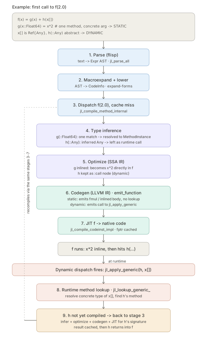
Flowchart of the Julia compilation pipeline: parse, lower, infer, optimize, codegen and JIT, with a statically dispatched call resolved and inlined at compile time and a dynamically dispatched call deferred to a runtime method lookup that triggers a second compilation on first execution.

The two columns at the bottom are the whole point of the type system: if inference can pin down a concrete method at compile time, the call becomes a direct branch (often inlined into the caller); if it cannot, the call survives as a runtime dispatch with a method-table lookup and — on first hit — a fresh compile. Most performance work in Julia is just moving more calls from the right column to the left.

CC BY-SA 4.0 Raye Kimmerer. Last modified: June 22, 2026.
Website built with Franklin.jl and the Julia programming language.